DDPM

11 minute read

Published: December 19, 2023

这是一段令人破防的代码。

class GaussianDiffusion:
    def __init__(
        self,
        timesteps=1000,
        beta_schedule='linear'
    ):
        self.timesteps = timesteps
        
        if beta_schedule == 'linear':
            betas = linear_beta_schedule(timesteps)
        elif beta_schedule == 'cosine':
            betas = cosine_beta_schedule(timesteps)
        else:
            raise ValueError(f'unknown beta schedule {beta_schedule}')
        self.betas = betas
            
        self.alphas = 1. - self.betas
        self.alphas_cumprod = torch.cumprod(self.alphas, axis=0)
        self.alphas_cumprod_prev = F.pad(self.alphas_cumprod[:-1], (1, 0), value=1.)
        
        # calculations for diffusion q(x_t | x_{t-1}) and others
        self.sqrt_alphas_cumprod = torch.sqrt(self.alphas_cumprod)
        self.sqrt_one_minus_alphas_cumprod = torch.sqrt(1.0 - self.alphas_cumprod)
        self.log_one_minus_alphas_cumprod = torch.log(1.0 - self.alphas_cumprod)
        self.sqrt_recip_alphas_cumprod = torch.sqrt(1.0 / self.alphas_cumprod)
        self.sqrt_recipm1_alphas_cumprod = torch.sqrt(1.0 / self.alphas_cumprod - 1)
        
        # calculations for posterior q(x_{t-1} | x_t, x_0)
        self.posterior_variance = (
            self.betas * (1.0 - self.alphas_cumprod_prev) / (1.0 - self.alphas_cumprod)
        )
        # below: log calculation clipped because the posterior variance is 0 at the beginning
        # of the diffusion chain
        self.posterior_log_variance_clipped = torch.log(self.posterior_variance.clamp(min =1e-20))
        
        self.posterior_mean_coef1 = (
            self.betas * torch.sqrt(self.alphas_cumprod_prev) / (1.0 - self.alphas_cumprod)
        )
        self.posterior_mean_coef2 = (
            (1.0 - self.alphas_cumprod_prev)
            * torch.sqrt(self.alphas)
            / (1.0 - self.alphas_cumprod)
        )
    
    # get the param of given timestep t
    def _extract(self, a, t, x_shape):
        batch_size = t.shape[0]
        out = a.to(t.device).gather(0, t).float()
        out = out.reshape(batch_size, *((1,) * (len(x_shape) - 1)))
        return out
    
    # forward diffusion (using the nice property): q(x_t | x_0)
    def q_sample(self, x_start, t, noise=None):
        if noise is None:
            noise = torch.randn_like(x_start)

        sqrt_alphas_cumprod_t = self._extract(self.sqrt_alphas_cumprod, t, x_start.shape)
        sqrt_one_minus_alphas_cumprod_t = self._extract(self.sqrt_one_minus_alphas_cumprod, t, x_start.shape)

        return sqrt_alphas_cumprod_t * x_start + sqrt_one_minus_alphas_cumprod_t * noise
    
    # Get the mean and variance of q(x_t | x_0).
    def q_mean_variance(self, x_start, t):
        mean = self._extract(self.sqrt_alphas_cumprod, t, x_start.shape) * x_start
        variance = self._extract(1.0 - self.alphas_cumprod, t, x_start.shape)
        log_variance = self._extract(self.log_one_minus_alphas_cumprod, t, x_start.shape)
        return mean, variance, log_variance
    
    # Compute the mean and variance of the diffusion posterior: q(x_{t-1} | x_t, x_0)
    def q_posterior_mean_variance(self, x_start, x_t, t):
        posterior_mean = (
            self._extract(self.posterior_mean_coef1, t, x_t.shape) * x_start
            + self._extract(self.posterior_mean_coef2, t, x_t.shape) * x_t
        )
        posterior_variance = self._extract(self.posterior_variance, t, x_t.shape)
        posterior_log_variance_clipped = self._extract(self.posterior_log_variance_clipped, t, x_t.shape)
        return posterior_mean, posterior_variance, posterior_log_variance_clipped
    
    # compute x_0 from x_t and pred noise: the reverse of `q_sample`
    def predict_start_from_noise(self, x_t, t, noise):
        return (
            self._extract(self.sqrt_recip_alphas_cumprod, t, x_t.shape) * x_t -
            self._extract(self.sqrt_recipm1_alphas_cumprod, t, x_t.shape) * noise
        )
    
    # compute predicted mean and variance of p(x_{t-1} | x_t)
    def p_mean_variance(self, model, x_t, t, clip_denoised=True):
        # predict noise using model
        pred_noise = model(x_t, t)
        # get the predicted x_0: different from the algorithm2 in the paper
        x_recon = self.predict_start_from_noise(x_t, t, pred_noise)
        if clip_denoised:
            x_recon = torch.clamp(x_recon, min=-1., max=1.)
        model_mean, posterior_variance, posterior_log_variance = \
                    self.q_posterior_mean_variance(x_recon, x_t, t)
        return model_mean, posterior_variance, posterior_log_variance
        
    # denoise_step: sample x_{t-1} from x_t and pred_noise
    @torch.no_grad()
    def p_sample(self, model, x_t, t, clip_denoised=True):
        # predict mean and variance
        model_mean, _, model_log_variance = self.p_mean_variance(model, x_t, t,
                                                    clip_denoised=clip_denoised)
        noise = torch.randn_like(x_t)
        # no noise when t == 0
        nonzero_mask = ((t != 0).float().view(-1, *([1] * (len(x_t.shape) - 1))))
        # compute x_{t-1}
        pred_img = model_mean + nonzero_mask * (0.5 * model_log_variance).exp() * noise
        return pred_img
    
    # denoise: reverse diffusion
    @torch.no_grad()
    def p_sample_loop(self, model, shape):
        batch_size = shape[0]
        device = next(model.parameters()).device
        # start from pure noise (for each example in the batch)
        img = torch.randn(shape, device=device)
        imgs = []
        for i in tqdm(reversed(range(0, timesteps)), desc='sampling loop time step', total=timesteps):
            img = self.p_sample(model, img, torch.full((batch_size,), i, device=device, dtype=torch.long))
            imgs.append(img.cpu().numpy())
        return imgs
    
    # sample new images
    @torch.no_grad()
    def sample(self, model, image_size, batch_size=8, channels=3):
        return self.p_sample_loop(model, shape=(batch_size, channels, image_size, image_size))
    
    # compute train losses
    def train_losses(self, model, x_start, t):
        # generate random noise
        noise = torch.randn_like(x_start)
        # get x_t
        x_noisy = self.q_sample(x_start, t, noise=noise)
        predicted_noise = model(x_noisy, t)
        loss = F.mse_loss(noise, predicted_noise)
        return loss

这个对初学者真的很不友好。我希望我这个废物可以看懂这些代码究竟在写什么，但是中间的 numpy 用法和 torch 用法有点太多了，所以我希望自己可以慢慢啃下来。

首先我们得先硬背下来 $\text{diffusion}$ 的各种参数定义，代码里的这一段：

        self.betas = betas
        self.alphas = 1. - self.betas
        self.alphas_cumprod = torch.cumprod(self.alphas, axis=0)
        self.alphas_cumprod_prev = F.pad(self.alphas_cumprod[:-1], (1, 0), value=1.)
        # calculations for diffusion q(x_t | x_{t-1}) and others
        self.sqrt_alphas_cumprod = torch.sqrt(self.alphas_cumprod)
        self.sqrt_one_minus_alphas_cumprod = torch.sqrt(1.0 - self.alphas_cumprod)
        self.log_one_minus_alphas_cumprod = torch.log(1.0 - self.alphas_cumprod)
        self.sqrt_recip_alphas_cumprod = torch.sqrt(1.0 / self.alphas_cumprod)
        self.sqrt_recipm1_alphas_cumprod = torch.sqrt(1.0 / self.alphas_cumprod - 1)

就是他定义的一堆参数。首先这个 betas 是外部传来的一个函数生成的，原始论文是直接线性生成的，但是后面有论文优化到用一个 cosine_beta_schedule 的东西生成。回忆一下，$\beta$ 就是前向过程中高斯噪声的参数：

\[q(\mathbf{x}_t \vert \mathbf{x}_{t-1}) = \mathcal{N}(\mathbf{x}_t; \sqrt{1 - \beta_t} \mathbf{x}_{t-1}, \beta_t\mathbf{I}) \\\]

这里不得不提一嘴，我们处理图片时已经把像素值正则化到 $[-1,1]$ 上了。

继续定义：

$\alpha=1-\beta,\bar{\alpha}t = \prod{i=1}^t \alpha_i$，所以论文里 $\bar{\alpha}$ 就是代码里的 alphas_cumprod。

我查询了一下 axis 参数的含义，发现和 dim 是一样的，有点奇怪。这两个可以混用吗？存疑。

破案了，torch 用 dim，numpy 用 axis，但是好像这个函数可以混用，疑似兼容了。

sqrt_alphas_cumprod_prev 就是它开根号。抽象的来了，alphas_cumprod_prev 是什么玩意？F 是 torch.nn.functional，让我们 $\text{GPT}$ 一下 F.pad。

torch.nn.functional.pad 是 PyTorch 深度学习框架中的一个功能，用于对张量（通常是多维数组）的边缘进行填充。这在深度学习中尤其有用，比如在卷积神经网络的操作中，你可能需要调整输入数据的尺寸。这个函数提供了灵活的方式来增加张量的维度。
torch.nn.functional.pad(input, pad, mode='constant', value=0)
input (Tensor): 要进行填充的输入张量。
pad (tuple): 定义填充量的元组。元组的长度是 2 倍的输入张量维数。> 例如，对于 4 维的张量，你需要 8 个值，形如 (pad_left, pad_right, pad_top, pad_bottom, pad_front, pad_back)。
mode (str): 填充模式。常用的模式包括 ‘constant’（常数填充，默认值为0）、’reflect’（反射填充）和 ‘replicate’（重复边缘值填充）。
value (float): 当模式为 ‘constant’ 时，用于填充的值。假设你有一个 2x3 的 2D 张量，你想在每个边上添加一个值的填充：
import torch
import torch.nn.functional as F
x = torch.tensor([[1, 2, 3],
                 [4, 5, 6]])
padded_x = F.pad(x, (1, 1, 1, 1), 'constant', value=0)
print(padded_x)
这将输出一个 4x5 的张量，原始张量的边缘被 0 填充。

感觉是在做 $\text{CNN}$ 会用到的东西…所以搞了半天其实就是平移了一下， $x[t]=\prod_{i=1}^{t-1} \alpha_i$，定义 $x[0]=1$。

sqrt_one_minus_alphas_cumprod 就是 $\sqrt{1-\bar{\alpha_t}}$，log_one_minus_alphas_cumprod 就是 $\ln{(1-\bar{\alpha_t})}$， sqrt_recip_alphas_cumprod 就是 $\frac 1{\sqrt{\bar{\alpha_t}}}$， sqrt_recipm1_alphas_cumprod？我猜 m1 是 minus 1 的意思，就是 $\sqrt{\frac 1{\bar{\alpha_t}}-1}$

$\text{recip}$ 是倒数的意思。

接下来的代码需要我们回顾一下 $\text{DDPM}$ 做的事情。

下面的内容纯属自己瞎编。

我的理解是：$\text{DDPM}$ 是一个有更多 $\text{latent variance}$ 的 $\text{VAE}$，其核心思想是：矩阵空间只有很少的符合某种分布的才能算是图片，我们通过构造潜变量，使得可以通过潜变量的后验分布（也就是在当前潜变量下原图的条件概率分布）采样出图片，而潜变量的后验分布可以用多层的高斯分布来拟合。而这个高斯分布，又可以用神经网络来预测。$\text{VAE}$ 只有一层拟合，而 $\text{DDPM}$ 有很多层，这可能是 $\text{diffusion}$ 吊打 $\text{VAE}$ 的一个原因。

这里我再瞎编一下，应该是 timestep 足够多的情况下，每一层的变化都不大，用高斯分布拟合误差会小，可以训练出来。

它的前向过程是把一张图片逐渐加噪声变成一个从标准正态分布中采样出来的高斯噪声，这样可以让我们通过一个高斯噪声按照后验分布采样出一张图（这样可以最接近原图像分布）。在原论文中，$q$ 表示前向过程的概率分布，$p_\theta$ 表示用高斯分布拟合得到的后验分布，也就是我们要训练的东西。

通过简单的推导有：

\[\mathbf{x}_t = \sqrt{\bar{\alpha}_t}\mathbf{x}_0 + \sqrt{1 - \bar{\alpha}_t}\mathbf{\epsilon}\]

也就是，前向过程只需要原图和一个采样出来的标准高斯噪声就可以了。也就是：

\[q(\mathbf{x}_t \vert \mathbf{x}_{0}) = \mathcal{N}(\mathbf{x}_t; \sqrt{\bar{\alpha}_t} \mathbf{x}_{0}, ({1 - \bar{\alpha}_t}\mathbf){I}) \\\]

反向过程假设已知 $\mathbf x_t$，$q(\mathbf{x}_{t-1}

\mathbf{x}t)$ 可被近似为一个高斯分布 $p\theta(\mathbf{x}{t-1} \vert \mathbf{x}_t) = \mathcal{N}(\mathbf{x}{t-1}; \boldsymbol{\mu}\theta(\mathbf{x}_t, t), \boldsymbol{\Sigma}\theta(\mathbf{x}_t, t))\$。

先往下看看代码：

    # get the param of given timestep t
    def _extract(self, a, t, x_shape):
        batch_size = t.shape[0]
        out = a.to(t.device).gather(0, t).float()
        out = out.reshape(batch_size, *((1,) * (len(x_shape) - 1)))
        return out
    # forward diffusion (using the nice property): q(x_t | x_0)
    def q_sample(self, x_start, t, noise=None):
        if noise is None:
            noise = torch.randn_like(x_start)

        sqrt_alphas_cumprod_t = self._extract(self.sqrt_alphas_cumprod, t, x_start.shape)
        sqrt_one_minus_alphas_cumprod_t = self._extract(self.sqrt_one_minus_alphas_cumprod, t, x_start.shape)

        return sqrt_alphas_cumprod_t * x_start + sqrt_one_minus_alphas_cumprod_t * noise

下面这段代码就是前向过程获取噪声。只不过，这个 _extract 函数是干啥的？看起来就是提取开始定义的 tensor 里的东西啊？然后这个函数也是一堆抽象的没见过的 py 用法，虽然是我太菜了。

torch.gather 是 PyTorch 中用于从输入张量中按指定索引收集值的函数。其参数包括三个主要部分：输入张量，索引张量和指定的维度。下面是它的基本用法和参数说明：
torch.gather(input, dim, index, out=None)
参数说明：
input：输入张量，从中收集值。
dim：一个整数，指定在哪个维度上进行收集操作。
index：包含索引的张量，用于确定在 dim 维度上收集哪些值。index 张量的形状必须与 input 张量的形状在维度 dim 之外的维度上是广播兼容的。通常，index 张量的数据类型应为整数类型。
out：可选参数，如果提供了此参数，将结果存储在指定的输出张量中。
示例：
import torch
# 创建一个输入张量
input_tensor = torch.tensor([[1, 2], [3, 4], [5, 6]])
# 创建一个索引张量
index_tensor = torch.tensor([[0, 1], [2, 0]])
# 在维度0上使用索引张量从输入张量中收集值
result = torch.gather(input_tensor, 0, index_tensor)
print(result)
tensor([[1, 4], [5, 2]])
在这个示例中，input_tensor 是一个形状为 (3, 2) 的张量，index_tensor 是一个形状为 (2, 2) 的张量。torch.gather 将根据 index_tensor 中的值，在维度 0 上从 input_tensor 中收集对应的值。结果将是一个形状为 (2, 2) 的张量。

它应该是将给定 tensor 的形状改成 index 的形状，然后值变成在原来 tensor 上给定的 dim 采样。相当于对 dim 这个维度进行缩减或者增加。

至于这个抽象的 * 运算：

*((1,) * (len(x_shape) - 1))

最外层的 * 是解压缩，相当于把整个元组解开扔进 reshape 的参数里，里面的 * 是重复 (len(x_shape) - 1) 次。

经过一番理解，我发现这个 _extract 函数可以提取出用来和 batch_size 张图片相乘的参数 tensor。为啥要这么做？因为每次丢进去的 batch_size 张图片的 t 可能都不一样。我们来看看训练时候的代码：

    t = torch.randint(0, timesteps, (batch_size,), device=device).long()
    loss = gaussian_diffusion.train_losses(model, images, t)

它的 t 都是直接随的，所以每一个 t 不一样就是了。虽然不知道为啥这么设计，不能每个 t 单独跑一次么？我猜是怕丢失信息吧，如果先训练 t=1，训练到 t=1000 可能 t=1 就白训练了。这下不得不感叹 torch.tensor 乘法的神奇了。

下面一段代码：

 def q_mean_variance(self, x_start, t):
    mean = self._extract(self.sqrt_alphas_cumprod, t, x_start.shape) * x_start
    variance = self._extract(1.0 - self.alphas_cumprod, t, x_start.shape)
    log_variance = self._extract(self.log_one_minus_alphas_cumprod, t, x_start.shape)
    return mean, variance, log_variance

这个就是纯返回系数 tensor，具体什么用我们往下看。

后面是计算优化目标了，也就是一堆公式。这里实在是没时间浪费笔墨去推导了，写几个看推导时候想到的一些东西吧：

第一步最大似然估计，然后是经典 $\text{VAE}$ 计算下界，也就是：枚举潜变量构造积分，然后分子分母同乘以构造出前向分布，再根据贝叶斯公式提取出一个 $\text{KL}$ 散度（或者直接琴生不等式，虽然我觉得前者更好，因为还能解释 $\text{VAE}$ 中先优化下界等价于最小化 $\text{KL}$ 散度的事情，好吧因为我才刚入门就不瞎说了）。
超长等式的第五行实在有点神仙，它用上了马尔可夫性，且基于以下这样的事实：
- 我们是求不出 $q(\mathbf{x}_{t-1} \vert \mathbf{x}_t)$ 的。这也好理解，我们肯定不知道当前的这个隐变量会偏向哪个最终图片，这绝对不是高斯分布（最多是估计，但我们现在不是在估计）。
- 但是如果在已知最终图片的情况下，也就是 $q(\mathbf{x}_{t-1} \vert \mathbf{x}_t, \mathbf{x}_0)$，我们可以求出来，也就是这玩意是一个高斯分布！经过暴推可以得到这是一个均值为
  \[\tilde\mu_t=\frac{\sqrt{\alpha_t}(1 - \bar{\alpha}_{t-1})}{1 - \bar{\alpha}_t} \mathbf{x}_t + \frac{\sqrt{\bar{\alpha}_{t-1}}\beta_t}{1 - \bar{\alpha}_t} \mathbf{x}_0\]
  方差为
  \[\tilde\beta_t=\frac{1 - \bar{\alpha}_{t-1}}{1 - \bar{\alpha}_t} \cdot \beta_t\]
  的高斯分布。注意 $\tilde\beta$ 后面还要用。
所以我们根据马尔可夫性把 $\mathbf x_0$ 也带上。
中间有一段突然把期望的分布改了，我还傻傻的想了半天为啥：

\[\begin{aligned} L &= \mathbb{E}_{q(\mathbf{x}_{1:T}\vert \mathbf{x}_{0})} \Big[ \log\frac{q(\mathbf{x}_T \vert \mathbf{x}_0)}{p_\theta(\mathbf{x}_T)} + \sum_{t=2}^T \log \frac{q(\mathbf{x}_{t-1} \vert \mathbf{x}_t, \mathbf{x}_0)}{p_\theta(\mathbf{x}_{t-1} \vert\mathbf{x}_t)} - \log p_\theta(\mathbf{x}_0 \vert \mathbf{x}_1) \Big] \\ &= \mathbb{E}_{q(\mathbf{x}_{T}\vert \mathbf{x}_{0})}\Big[\log\frac{q(\mathbf{x}_T \vert \mathbf{x}_0)}{p_\theta(\mathbf{x}_T)}\Big]+\sum_{t=2}^T \mathbb{E}_{q(\mathbf{x}_{t}, \mathbf{x}_{t-1}\vert \mathbf{x}_{0})}\Big[\log \frac{q(\mathbf{x}_{t-1} \vert \mathbf{x}_t, \mathbf{x}_0)}{p_\theta(\mathbf{x}_{t-1} \vert\mathbf{x}_t)}\Big] - \mathbb{E}_{q(\mathbf{x}_{1}\vert \mathbf{x}_{0})}\Big[\log p_\theta(\mathbf{x}_0 \vert \mathbf{x}_1)\Big]\end{aligned}\]

其实是显然的，因为这个分布本身就是 $T+1$ 重的联合概率分布，然后里面的东西都和其他潜变量无关了，当然可以拿走（积分号提出去，全是 $1$）。具体的其实就是：

\[\int\mathrm d\mathbf x_1\int\mathrm d\mathbf x_2\cdots\int\mathrm d\mathbf x_T\log\frac{q(\mathbf{x}_T \vert \mathbf{x}_0)}{p_\theta(\mathbf{x}_T)}q(\mathbf{x}_{1:T}\vert \mathbf{x}_{0})\] \[=\int\mathrm d\mathbf x_1\int\mathrm d\mathbf x_2\cdots\int\mathrm d\mathbf x_T\log\frac{q(\mathbf{x}_T \vert \mathbf{x}_0)}{p_\theta(\mathbf{x}_T)}q(\mathbf{x}_{T}|\mathbf{x}_0)q(\mathbf{x}_{1:T-1}|\mathbf{x}_{T},\mathbf{x}_0)\] \[=\int\mathrm d\mathbf x_T\log\frac{q(\mathbf{x}_T \vert \mathbf{x}_0)}{p_\theta(\mathbf{x}_T)}q(\mathbf{x}_{T}|\mathbf{x}_0)\int\mathrm d\mathbf x_1\int\mathrm d\mathbf x_2\cdots\mathrm d\mathbf x_{T-1} q(\mathbf{x}_{1:T-1}|\mathbf{x}_{T},\mathbf{x}_0)\] \[=\int\mathrm d\mathbf x_T\log\frac{q(\mathbf{x}_T \vert \mathbf{x}_0)}{p_\theta(\mathbf{x}_T)}q(\mathbf{x}_{T}|\mathbf{x}_0)\]

感觉是废话，我却想了半天，唉。

然后继续就是：

\[\begin{aligned}\\ &= \mathbb{E}_{q(\mathbf{x}_{T}\vert \mathbf{x}_{0})}\Big[\log\frac{q(\mathbf{x}_T \vert \mathbf{x}_0)}{p_\theta(\mathbf{x}_T)}\Big]+\sum_{t=2}^T \mathbb{E}_{q(\mathbf{x}_{t}\vert \mathbf{x}_{0})}\Big[q(\mathbf{x}_{t-1} \vert \mathbf{x}_t, \mathbf{x}_0)\log \frac{q(\mathbf{x}_{t-1} \vert \mathbf{x}_t, \mathbf{x}_0)}{p_\theta(\mathbf{x}_{t-1} \vert\mathbf{x}_t)}\Big] - \mathbb{E}_{q(\mathbf{x}_{1}\vert \mathbf{x}_{0})}\Big[\log p_\theta(\mathbf{x}_0 \vert \mathbf{x}_1)\Big] \\ &= \underbrace{D_\text{KL}(q(\mathbf{x}_T \vert \mathbf{x}_0) \parallel p_\theta(\mathbf{x}_T))}_{L_T} + \sum_{t=2}^T \underbrace{\mathbb{E}_{q(\mathbf{x}_{t}\vert \mathbf{x}_{0})}\Big[D_\text{KL}(q(\mathbf{x}_{t-1} \vert \mathbf{x}_t, \mathbf{x}_0) \parallel p_\theta(\mathbf{x}_{t-1} \vert\mathbf{x}_t))\Big]}_{L_{t-1}} -\underbrace{\mathbb{E}_{q(\mathbf{x}_{1}\vert \mathbf{x}_{0})}\log p_\theta(\mathbf{x}_0 \vert \mathbf{x}_1)}_{L_0} \end{aligned}\]

然后就构造出了两个神奇的 $\text{KL}$ 散度。我们来看看似然估计的意义是什么：$L_T$ 是前向过程得到的操作，也就是加噪声过程得到的噪声的概率分布和我们反向过程开始取的噪声的分布的接近程度。中间虽然也套了一个期望，但由于前向分布是一个简单的高斯分布，所以一堆 $\sum$ 得到的值也是清晰的，就是潜变量的接近程度的和嘛！也就是，基于高斯分布近似的去噪过程要尽可能接近真实的后验分布。$L_0$ 有点抽象，但其实表达的是最后一步生成出 $\mathrm x_0$ 的可能性，当然是越大越好。所以其实似然估计得到的东西是很符合直觉的。事实上，很多 $\text{Loss}$ 的推导都是基于似然估计，然后得到的也都是 $\text{KL}$ 散度相关的结果。

接下来的问题是，这么多散度怎么计算？论文里的处理方式是：

因为 $p_\theta$ 和前向过程得到的结果和训练无关，前者就是标准正态分布，后者基本就是标准正态分布，所以直接取 $0$。

中间的肯定不能去掉。因为两个都是高斯分布，直接调用高斯分布的 $\text{KL}$ 散度公式。为了计算方便，我们令协方差矩阵是对角矩阵（也就是像素变量是独立的，这个 $\text{VAE}$ 里也是这么处理的）。原始论文中让神经网络只输出期望，因为它固定了方差，$p_\theta(\mathrm x_{t-1}

\mathrm x_{t-1})$ 和 $q(\mathbf{x}{t-1} \vert \mathbf{x}_t, \mathbf{x}_0)=\tilde\beta{\mathbf t}$ 的方差完全一样，也方便计算。代入公式以后就是：

\[\frac1{2\tilde\beta_t^2}||\Delta\mu||^2\]

这里是两个分布的均值的二范数。那么式子就变得非常之简单了。

最后一部分论文是使用了离散的方法计算，也就是枚举 $[0,255]$ ，用求和代替积分，只能说有点抽象，但也很天才。

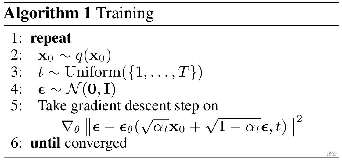
这样，$\text{DDPM}$ 的 $\text{Loss}$ 函数构建完毕！结果我往下翻还没完，说实话有点破防，这种预测均值的事实上效果不是最好的，论文里有另一种方式，也是一个很牛逼、越想越妙的方法：预测图片，肯定比预测噪声难！所以我们考虑把噪声预测出来！我们知道 $\mathbf x_t$ 的话，可以和 $\mathbf x_0$ 建立联系。由于懒，我直接把公式搞下来吧：

根据前面得到的前向过程我们有：

\[\mathbf{x_t}(\mathbf{x_0},\mathbf{\epsilon})=\sqrt{\bar{\alpha}_t}\mathbf{x}_0 + \sqrt{1 - \bar{\alpha}_t}\mathbf{\epsilon} \quad \text{ where } \mathbf{\epsilon}\sim \mathcal{N}(\mathbf{0}, \mathbf{I}) \\\]

所以我们把 $\epsilon$ 预测出来，顺带可以预测出一个 $\mathbf x_0$ ！将这个公式带入上述优化目标（注意这里的损失我们引入了潜变量 $\mathbf{x}_0,\epsilon$ ，所以需要再求一个数学期望），可以得到：

\[\begin{aligned} L_{t-1}&=\mathbb{E}_{\mathbf{x}_{0}}\Big(\mathbb{E}_{q(\mathbf{x}_{t}\vert \mathbf{x}_{0})}\Big[ \frac{1}{2{\tilde\beta_t^2}}\|\tilde{\boldsymbol{\mu}}_t(\mathbf{x}_t, \mathbf{x}_0) - {\boldsymbol{\mu}_\theta(\mathbf{x}_t, t)} \|^2\Big]\Big) \\ &=\mathbb{E}_{\mathbf{x}_{0},\mathbf{\epsilon}\sim \mathcal{N}(\mathbf{0}, \mathbf{I})}\Big[ \frac{1}{2{\tilde\beta_t^2}}\|\tilde{\boldsymbol{\mu}}_t\Big(\mathbf{x_t}(\mathbf{x_0},\mathbf{\epsilon}), \frac{1}{\sqrt{\bar \alpha_t}} \big(\mathbf{x_t}(\mathbf{x_0},\mathbf{\epsilon}) - \sqrt{1 - \bar{\alpha}_t} \mathbf{\epsilon} \big)\Big ) - {\boldsymbol{\mu}_\theta(\mathbf{x_t}(\mathbf{x_0},\mathbf{\epsilon}), t)} \|^2\Big] \\ &=\mathbb{E}_{\mathbf{x}_{0},\mathbf{\epsilon}\sim \mathcal{N}(\mathbf{0}, \mathbf{I})}\Big[ \frac{1}{2{\tilde\beta_t^2}}\|\Big (\frac{\sqrt{\alpha_t}(1 - \bar{\alpha}_{t-1})}{1 - \bar{\alpha}_t} \mathbf{x}_t(\mathbf{x_0},\mathbf{\epsilon}) + \frac{\sqrt{\bar{\alpha}_{t-1}}\beta_t}{1 - \bar{\alpha}_t} \frac{1}{\sqrt{\bar \alpha_t}} \big(\mathbf{x_t}(\mathbf{x_0},\mathbf{\epsilon}) - \sqrt{1 - \bar{\alpha}_t} \mathbf{\epsilon} \big) \Big) - {\boldsymbol{\mu}_\theta(\mathbf{x_t}(\mathbf{x_0},\mathbf{\epsilon}), t)} \|^2\Big] \\ &=\mathbb{E}_{\mathbf{x}_{0},\mathbf{\epsilon}\sim \mathcal{N}(\mathbf{0}, \mathbf{I})}\Big[ \frac{1}{2{\tilde\beta_t^2}}\|\frac{1}{\sqrt{\alpha_t}}\Big( \mathbf{x}_t(\mathbf{x_0},\mathbf{\epsilon}) - \frac{\beta_t}{\sqrt{1 - \bar{\alpha}_t}}\mathbf{\epsilon}\Big) - {\boldsymbol{\mu}_\theta(\mathbf{x_t}(\mathbf{x_0},\mathbf{\epsilon}), t)} \|^2\Big] \end{aligned}\\\]

我们不预测均值了，直接预测噪声，把 $\mu_\theta$ 扔了。新的均值可以用噪声表示，这里网上文章都跳步了，我详细写一下：

预测出的 $\mathbf x_0$ 是：

\[\mathbf x_0=\frac 1{\sqrt{\bar{\alpha}_t}}(\mathbf{x_t}(\mathbf{x_0},\mathbf{\epsilon})-\sqrt{1-\bar{\alpha}_t}\epsilon_\theta\mathbf({x}_t(\mathbf{x_0},\mathbf{\epsilon}))\]

然后是一个玄幻的操作，直接把 $\mu_\theta$ 换成 $\tilde\mu$ ，虽然不知道其他的会不会更好。最后式子变成：

\[\begin{aligned} &=\mathbb{E}_{\mathbf{x}_{0},\mathbf{\epsilon}\sim \mathcal{N}(\mathbf{0}, \mathbf{I})}\Big[ \frac{\beta_t^2}{2{\sigma_t^2}\alpha_t(1-\bar{\alpha}_t)}\| \mathbf{\epsilon}- \mathbf{\epsilon}_\theta\big(\mathbf{x}_t, t\big)\|^2\Big] \end{aligned}\\\]

论文又做了一个简化操作，舍去了前面的系数，因为在 $t$ 较大或者较小的时候，前面系数会很极端，所以为了稳定的训练，我们舍去系数。这就得到了论文里最最经典的 $\text{Loss}$ 函数：

Alt text

有一个问题，$\text{Loss}$ 不应该是所有的 $L_{t-1}$ 求和吗？为什么这里只写了一个？因为事实上这里有一个期望，所以我们可以训练的时候对于一个 batch 算和，然后把它当做期望。（感觉挺逆天的）

结果推了这么久的 $\text{Loss}$ 函数得到了一个这么显然的东西？甚至省去了 $L_0$！~~这就是菜逼克高手吗？~~所以学习这个东西，就是图个成就感。

然后我们来看看生成：

Alt text

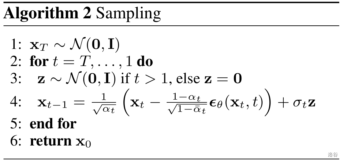
这也简单了。我们预测的是前向过程的噪声，所以直接反推出 $\mathbf x_0$ 再取样一个高斯噪声，然后代入 $q(\mathbf x_{t-1}

\mathbf x_0,\mathbf x_t)$ 进行采样，就可以推出这个代码了。

至于为什么不取均值？我们本身就是得到概率分布，当然采样会符合要求。这样也能加强模型的随机性，不然可能效果还会很差。

至此，$\text{DDPM}$ 的原理部分就完全结束了。

说了一堆废话，继续看代码，之前留着没看的定义：

	# calculations for posterior q(x_{t-1} | x_t, x_0)     
	self.posterior_variance = (
            self.betas * (1.0 - self.alphas_cumprod_prev) / (1.0 - self.alphas_cumprod)
        )
        # below: log calculation clipped because the posterior variance is 0 at the beginning
        # of the diffusion chain
        self.posterior_log_variance_clipped = torch.log(self.posterior_variance.clamp(min =1e-20))
        
        self.posterior_mean_coef1 = (
            self.betas * torch.sqrt(self.alphas_cumprod_prev) / (1.0 - self.alphas_cumprod)
        )
        self.posterior_mean_coef2 = (
            (1.0 - self.alphas_cumprod_prev)
            * torch.sqrt(self.alphas)
            / (1.0 - self.alphas_cumprod)
        )

显然这是 $q(\mathbf x_{t-1}

\mathbf x_0,\mathbf x_{t})$ 的那几个算方差和均值的系数。

它还保存了一个 log 的方差，不知道干啥，先往下看。

torch.clamp 相当于一个 clip 操作，防止对 0 取负数。

    def q_posterior_mean_variance(self, x_start, x_t, t):
        posterior_mean = (
            self._extract(self.posterior_mean_coef1, t, x_t.shape) * x_start
            + self._extract(self.posterior_mean_coef2, t, x_t.shape) * x_t
        )
        posterior_variance = self._extract(self.posterior_variance, t, x_t.shape)
        posterior_log_variance_clipped = self._extract(self.posterior_log_variance_clipped, t, x_t.shape)
        return posterior_mean, posterior_variance, posterior_log_variance_clipped
    

这是把它直接算出来了。

    def predict_start_from_noise(self, x_t, t, noise):
        return (
            self._extract(self.sqrt_recip_alphas_cumprod, t, x_t.shape) * x_t -
            self._extract(self.sqrt_recipm1_alphas_cumprod, t, x_t.shape) * noise
        )

这就是估计 $\mathbf x_0$ ！

    def p_mean_variance(self, model, x_t, t, clip_denoised=True):
        # predict noise using model
        pred_noise = model(x_t, t)
        # get the predicted x_0: different from the algorithm2 in the paper
        x_recon = self.predict_start_from_noise(x_t, t, pred_noise)
        if clip_denoised:
            x_recon = torch.clamp(x_recon, min=-1., max=1.)
        model_mean, posterior_variance, posterior_log_variance = \
                    self.q_posterior_mean_variance(x_recon, x_t, t)
        return model_mean, posterior_variance, posterior_log_variance

又包装了一层，不过这里有一个超参数，表示要不要对预测出来的 $\mathrm x_0$ 进行 clip 处理。反正就是一个框架，调用一下返回之前所有东西。

    def p_sample(self, model, x_t, t, clip_denoised=True):
        # predict mean and variance
        model_mean, _, model_log_variance = self.p_mean_variance(model, x_t, t,
                                                    clip_denoised=clip_denoised)
        noise = torch.randn_like(x_t)
        # no noise when t == 0
        nonzero_mask = ((t != 0).float().view(-1, *([1] * (len(x_t.shape) - 1))))
        # compute x_{t-1}
        pred_img = model_mean + nonzero_mask * (0.5 * model_log_variance).exp() * noise
        return pred_img

看到这里就知道了，原来这个 $\log$ 是方便计算用的。

这个 nonzero_mask 是干啥的？这就是特判 t=0 的情况，如果是 $0$ 就不采样，否则采样。虽然我也不知道为啥他要这么写而不是用 if…

    def p_sample_loop(self, model, shape):
        batch_size = shape[0]
        device = next(model.parameters()).device
        # start from pure noise (for each example in the batch)
        img = torch.randn(shape, device=device)
        imgs = []
        for i in tqdm(reversed(range(0, timesteps)), desc='sampling loop time step', total=timesteps):
            img = self.p_sample(model, img, torch.full((batch_size,), i, device=device, dtype=torch.long))
            imgs.append(img.cpu().numpy())
        return imgs

看到这里就 easy 了。这就是推理过程的代码版。tqdm 是进度条，虽然我不会用，但是我看得懂（不是）。

    def train_losses(self, model, x_start, t):
        # generate random noise
        noise = torch.randn_like(x_start)
        # get x_t
        x_noisy = self.q_sample(x_start, t, noise=noise)
        predicted_noise = model(x_noisy, t)
        loss = F.mse_loss(noise, predicted_noise)
        return loss

这就是废话，预测出来算一个 mse。

偶天哪，终于看懂了（悲伤），花费不知道多久。

后记：

其实我一直非常非常的好奇，直接把过程中得到的 $\mathbf x_0$ 输出会怎么样。

我拿 cifar10 试了一下（好吧其实就是魔改代码），训练了 $50$ 个 $\text{epoch}$，首先随便生 $64$ 个图，效果是这样的：

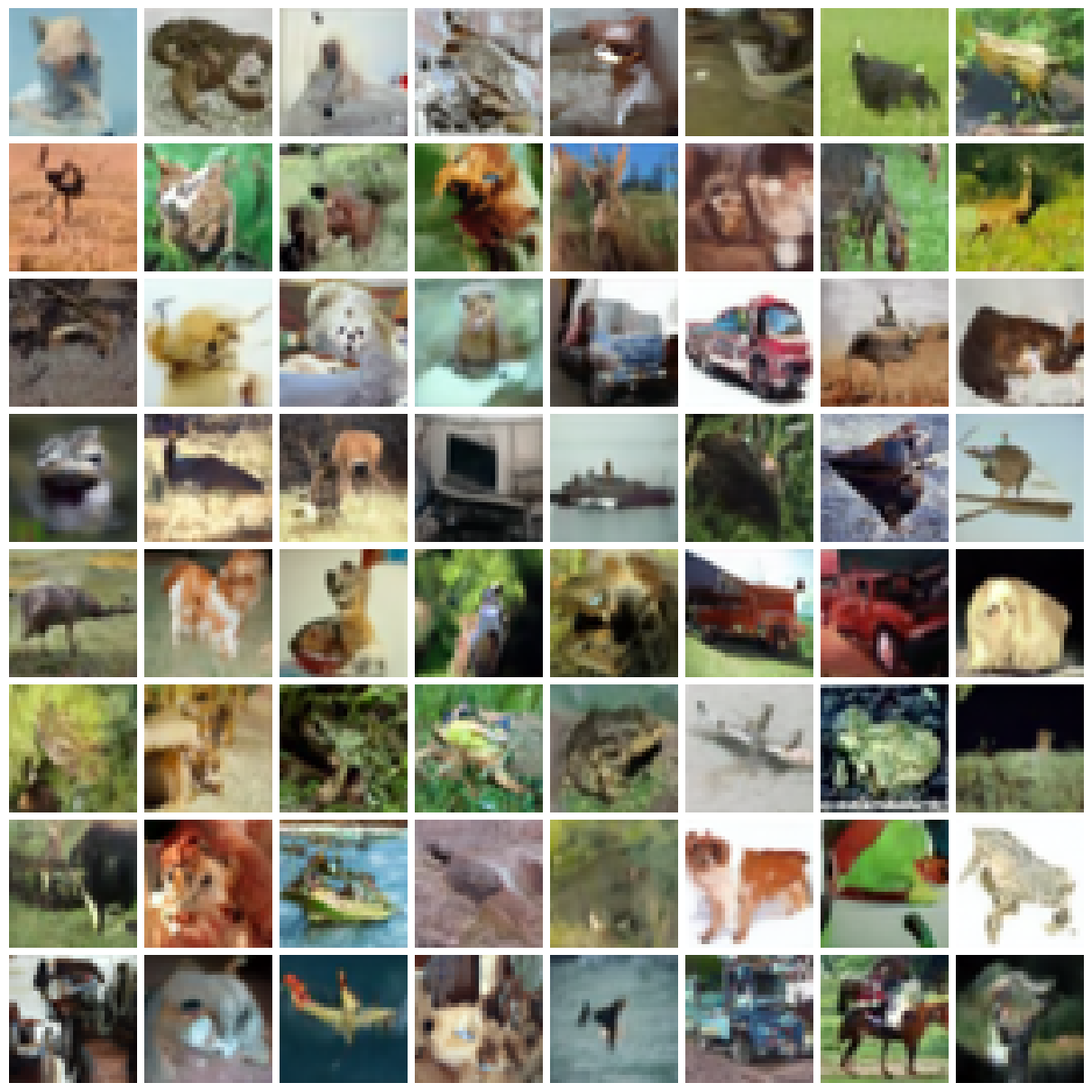
取了中间那个很好看的货车。然后我查看了一下最后 $64$ 步的降噪过程，效果是这样的：

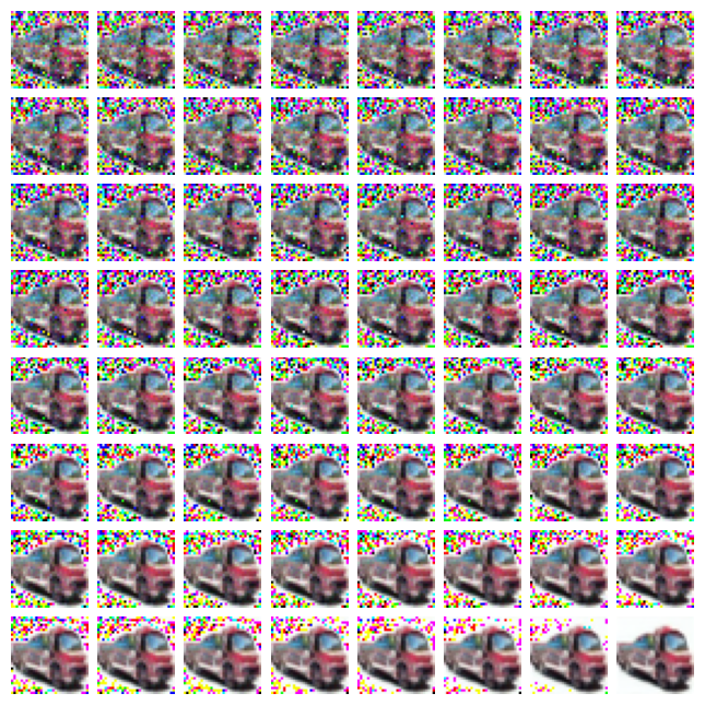
输出中间的 $\mathbf x_0$，代码（省去一堆 ipynb 里的）

fig = plt.figure(figsize=(12, 12), constrained_layout=True)
gs = fig.add_gridspec(16, 16)
for i in range(64):
    f_ax = fig.add_subplot(gs[i//8, i%8])
    t = torch.full((64,), 999-15*i, device=device).long()
    ori = torch.from_numpy(generated_images[15*i]).to(device)
    pred_noise = model(ori, t)
    with torch.no_grad():
        x_recon = gaussian_diffusion.predict_start_from_noise(ori, t, pred_noise).to('cpu').numpy()
        img = x_recon[21].reshape(3, 32, 32).transpose([1, 2, 0])
        f_ax.imshow(np.array((img+1.0) * 255 / 2, dtype=np.uint8))
        f_ax.axis("off")

为啥这么一点点代码都调了这么久（哭泣）

效果是这样的：

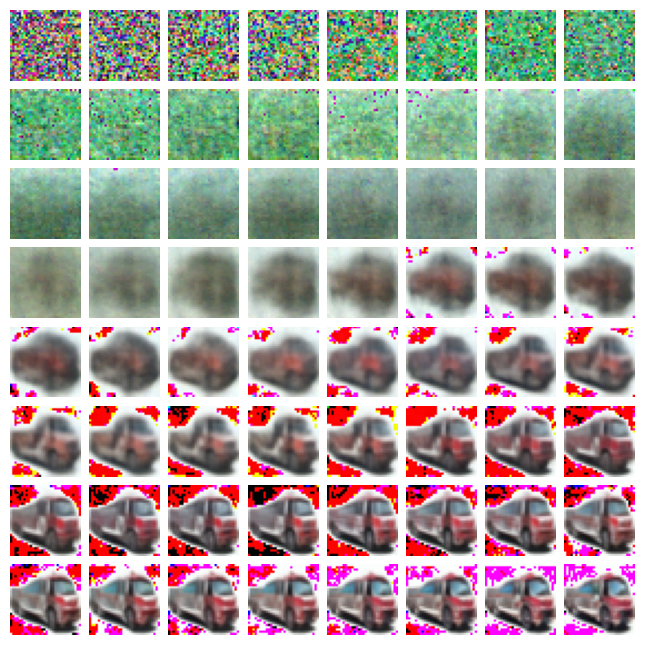
太抽象了，这一点也不绿啊，为啥前面预测出来都是绿的…我把最后 $64$ 步输出来，效果是这样的：

看来真的，很有趣啊，emmm，真的误差一点一点减小了。

Share on

Twitter Facebook LinkedIn

Ji Xie

DDPM

后记：

Share on

You May Also Enjoy

Diffusers

Linear Algebra Done Right

Mathematics Analysis Review

Linear-Algebra-Review